An Introduction to Publishing with R Markdown
What is R Markdown, how will it help you to create and publish reproducible research, and how do you get started...
- A Case for Reproducible Workflows
- What is R Markdown?
- Creating and Running R Markdown
- Rendering Process
- Conclusion
I recently completed a course that used R for various statistical and machine learning methods. In a separate article I have discussed the course and my semester project, Text Sentiment Analysis with R. Another is coming soon with R Markdown tips and tricks I learned along the way. But first some background is in order…
A Case for Reproducible Workflows
In this article I’ll provide a simple introduction to the R Markdown for the uninitiated. I consider this approach, a form of single source publishing, a vital component of reproducible computational research, and an essential skill. The following short video dramatization of real-life events provides a motivating example that we can all relate to… (Link opens in YouTube)
The video ends with the glimpse of a better future, a hopeful vision of reproducible workflows powered by source control (git) and R Markdown. It is within reach! The tools are built into RStudio and the essentials are easy to grasp and apply. The short time it takes to begin using this method will pay generous dividends ever after.
As this post grew and grew, I felt like the initial promise of a solution “within reach” seemed less and less credible. Perhaps after writing and digesting this I will be able to return to the topic and create the TL;DR version…
What is R Markdown?
R Markdown was introduced in 2012 by Yihui Xie, who has authored many of the most important packages in this space, including {knitr}. In his book, R Markdown: The Definitive Guide, Xie describes R Markdown as “an authoring framework for data science,” in which a single .Rmd file is used to “save and execute code, and generate high quality reports” automatically. A very wide range of document types and formats are supported, including documents and presentations in HTML, PDF, Word, Markdown, Powerpoint, LaTeX, and more. Homework assignments, journal articles, full-length books, formal reports, presentations, web pages, and interactive dashboards are just some of the possibilities he describes, with examples of each. To say it is a flexible and dynamic ecosystem is an understatement.
R Markdown Syntax
Anyone that has worked with R Markdown’s Python equivalent, Jupyter Notebooks, will find the following familiar. You may also be interested in my article Exploring Jupyter Notebook-Based Research.
R Markdown files consist of the following elements:
- A metadata header that sets various output options, using the YAML syntax
- Body text that is formatted in Markdown
- Interspersed code chunks that are set off by three backticks and a curly braced block that specifies the language used and sets chunk options
R Markdown also allows users to embed code expressions in the prose by enclosing them in single backticks.
Sample Code and Output
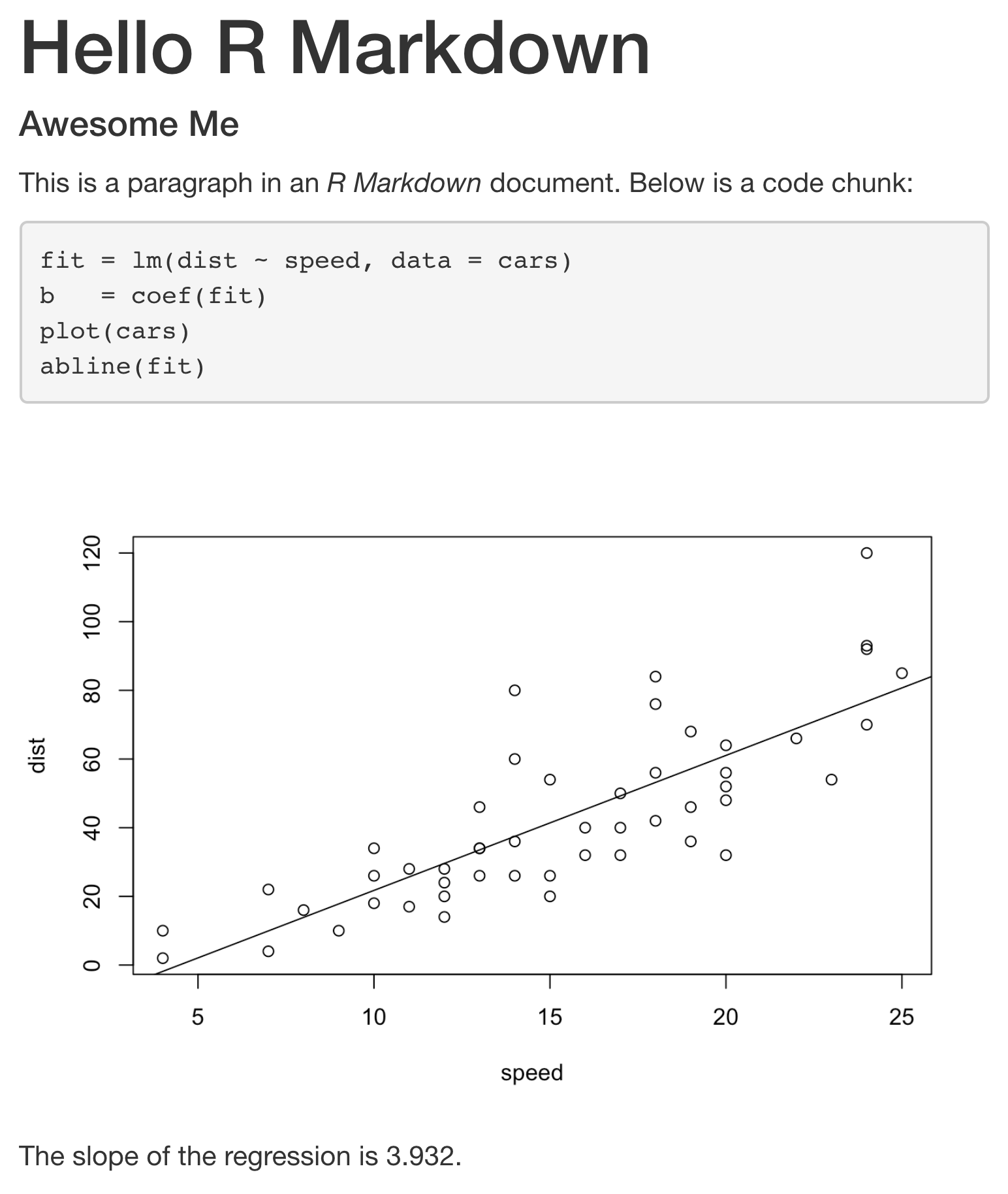
A minimal .Rmd example is included below. This is based on the Xie’s sample, which I’ve modified to demonstrate all of the elements mentioned above.
01: ---
02: title: "Hello R Markdown"
03: author: "Awesome Me"
04: output: html_document
05: ---
06:
07: This is a paragraph in an _R Markdown_ document.
08: Below is a code chunk:
09:
10: ```{r fit-plot, echo=TRUE}
11: fit = lm(dist ~ speed, data = cars)
12: b   = coef(fit)
13: plot(cars)
14: abline(fit)
15: ```
16:
17: The slope of the regression is `r round(b[2], digits = 3)`.
Let’s take a moment to walk through this, line by line.
- Lines 01 through 05 are the YAML header (aka frontmatter), delimited above and below by lines containing three dashes. Here, we’ve specified the document’s title and author, which are used to generate a header in the rendered output. Other options like date and subtitle are also available. Also specified is the default output type,
html_document. This section is actually optional, though rarely omitted. When it is, documents are rendered to HTML. More on YAML after the more pressing matters that follow. - Lines 07 and 08 are the body text (aka prose or narrative). The bit
_R Markdown_is an example of Markdown syntax, causing the text enclosed in underbar characters to be rendered in italics. A few quirks aside (e.g. newlines are considered spaces), the rest of the Markdown syntax is similarly straightforward, but surprisingly capable. - Lines 10 through 15 are an R code chunk, delimited by three backticks (
```)- Line 10 includes
{r fit-plot, echo=TRUE}, which specifies the language for this code block (R) and the chunk name (fit-plot). It also sets a chunk optionecho=TRUE, specifying that both the code and result will be included in the rendered output. - Lines 11 through 14 are standard R code
- Line 15 closes the code chunk
- Line 10 includes
- Line 17 is body text with an inline R expression. This expression will be evaluated when the document is rendered and the result will be included in the resulting output.
Rendering this code to an HTML file via the Knit button results in the following:
Creating and Running R Markdown
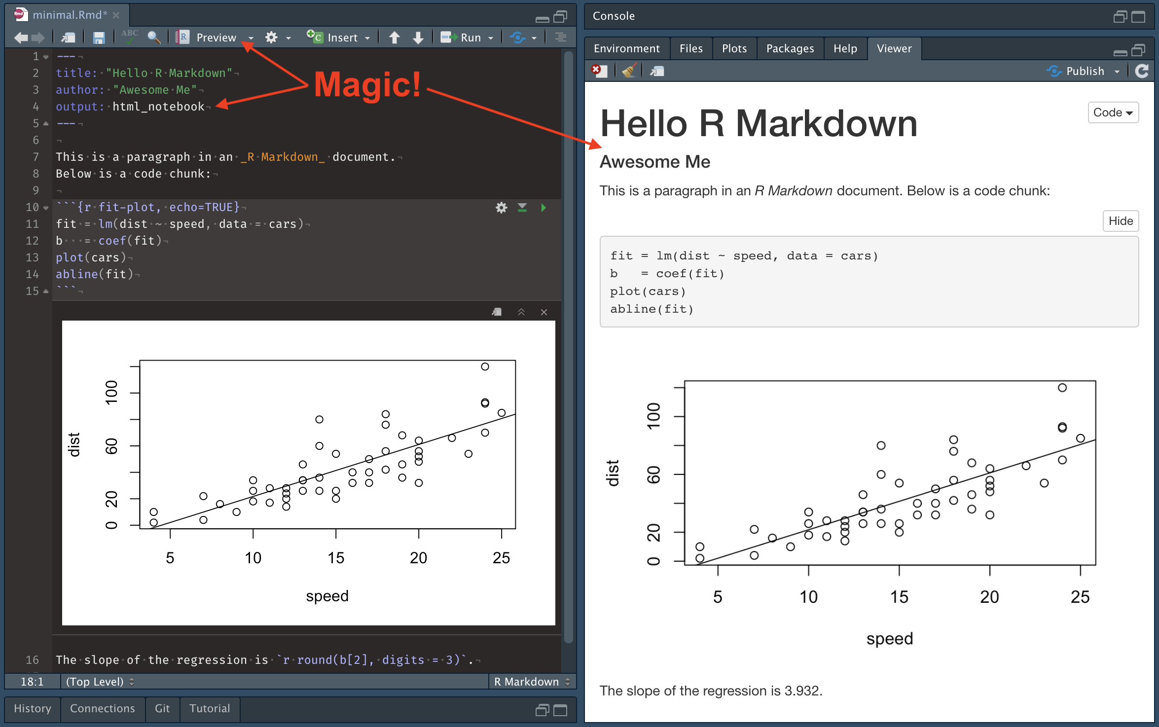
In RStudio, .Rmd files can be created from the File menu, by selecting New File... and then R Notebook. A template .Rmd will be opened, containing a YAML header, some body text, and a few code chunks to get you started.
Add chunks either by typing the backtick and curly brace syntax directly, using Insert on the editor toolbar, or with the keyboard shortcut Cmd/Ctrl + Alt + I. Pro-tip: this can also be used to ![]() SPLIT existing chunks!
SPLIT existing chunks!![]()
The difference between an .Rmd file and an R Notebook is subtle but important. In the context of RStudio, R Notebooks should be thought of as a particular interface for .Rmd files. This interface is triggered whenever html_notebook is the default (first or only) output specified, which is the case for any newly created R Notebook.
Note the important distinction between the output types
html_notebook, which enables the R Notebook Preview features, andhtml_document, which specifies a Knit output target.
The R Notebook interface provides three primary benefits.
- Code chunks can be executed independently and interactively.
- Click the green triangle button on the chunk toolbar or use
Cmd/Ctrl + Shift + Enterto run the current chunk. - Use
Cmd/Ctrl + Enterto run the current/selected line/lines. - Additional options including
Run AllandRun All Chunks Aboveare available from theRunmenu in the editor toolbar.
- Click the green triangle button on the chunk toolbar or use
- The output of each code chunk is displayed inline, just below the input.
- Chunk options are used control the contents and style of the output of individual chunks. For example, you can choose to hide the text output and control the aspect ratio of a figure generated.
- The output cells can be cleared or collapsed using controls in the upper right corner of the output or via the gear menu in the editor toolbar, next to the Preview button.
- Automatically updated HTML Previews!
-
Previewreplaces theKnitbutton on the editor toolbar when using the R Notebook interface. Clicking it displays an HTML preview in the Viewer pane. - This last point bears further discussion…
-
Ordinary R Markdown documents are “knitted,” but notebooks are “previewed.” While the notebook preview looks similar to a rendered R Markdown document, the notebook preview does not execute any of your R code chunks. It simply shows you a rendered copy of the Markdown output of your document along with the most recent chunk output. This preview is generated automatically whenever you save the notebook.
In short, create a new R Notebook, click Preview, make changes to the Notebook, save the changes, and violà! Finish your work, using the automatic Previews to guide your edits. Then Knit to the desired final format(s) using the drop down list on the Preview button.
This is a huge time-saver. When Knit is used to render final output the entire Notebook is run from scratch. Depending on its contents this can take a while, but even simple Notebooks take several seconds to process. By contrast, the Preview HTML is generated incrementally, as each change is made, and updated instantly with each save.
The result is not usually a true WYSIWYG experience due to differences between the way HTML and your final output format is rendered (e.g., HTML doesn’t have page breaks), but saves countless round-trips through the Knit-check-edit process. An added benefit of this approach is accelerated learning, greater willingness to experiment, etc., all engendered by the reduced friction that comes with near-instantaneous feedback.
Rendering Process
Clicking the Knit button kicks off the following process:
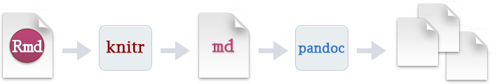
In a nutshell, R Markdown stands on the shoulders of knitr and Pandoc. The former executes the computer code embedded in Markdown, and converts R Markdown to Markdown. The latter renders Markdown to the output format you want (such as PDF, HTML, Word, and so on). - Xie, Preface
While it is not typically necessary to understand the details of this process it it useful to know that both knitr and Pandoc are involved. It is, however, critical to understand the following:
Under the hood, RStudio calls the function
rmarkdown::render()to render the document in a new R session. Please note the emphasis here, which often confuses R Markdown users. Rendering an Rmd document in a new R session means that none of the objects in your current R session (e.g., those you created in your R console) are available to that session. - Xie, Compile an R Markdown document
In other words your .Rmd must run start to finish, without errors, from a clean environment. If, for example, the code relies on variables created or packages loaded via the console during your interactive session, the Knit will fail. This requirement goes a long way to ensuring that others, given the same file, will get the same results. For more details, follow the link in the quote above.
Troubleshooting
To confirm that your .Rmd runs cleanly, perform the following steps:
- From RStudio’s
Sessionmenu, chooseClear Workspace.... In the dialog box that follows, confirm that the option “Include hidden objects” is ticked and click Yes. This clears your environment. - Return to the
Sessionmenu and chooseRestart R and Run All Chunks. This starts a fresh R session and runs the entire notebook, start to finish.
As an alternative to the first step you can include rm(list=ls()) at the top of your code. I believe this achieves an equivalent result, removing all objects in the current workspace. With that addition, simply use Restart R and Run All Chunks to reinitialize the R kernel and run your code, which will automatically clear the environment.
Finally, if Knit or Run All Chunks is failing in a way you don’t understand, step through the code. After clearing the workspace choose Restart R and Clear Output in the Session menu. Now use the methods described in [Running Files], above, to run each chunk until you find the problem. To isolate issues within a problematic chunk, break it into multiple chunks and/or run it line by line.
Any missing dependencies that would halt the Knit process should be identified by these methods.
Conclusion
It’s (way past?) time to draw this to a close. I hope that it has given you a grasp, or at least a taste, of:
- The value of reproducible research
- The important role that tools like R Markdown and R Notebook play in supporting reproducible research by combining prose, code, output, and supporting materials in a single document
- The syntaxes used in
.Rmdfiles, including YAML, Markdown, and code chunks - The concept that R Notebooks provide a way to interact with
.Rmdfiles - How to use Preview mode in R Notebooks to efficiently create great looking reports and improve your results
- How to render final output using Knit and how to troubleshoot problems that may arise
- The fundamental mechanics involved so you can at least ask informed questions when something isn’t working or you need to learn more
- Links to valuable resources when that time comes
If you learned half as much reading this as I learned creating it then we’re both doing well!
Further Reading
You could write a book about this. In fact, people have. Several…
This article relied heavily on Yihui Xie’s R Markdown: The Definitive Guide, specific sections of which have been linked throughout. In addition, it is hard to go wrong with any of his books, most of which are available online for free, and in print:
- Xie, Yihui, Alison Presmanes Hill, et al. Blogdown: Creating Websites with R Markdown. CRC Press, 2017. Google Books, https://bookdown.org/yihui/blogdown/.
- Xie, Yihui. Bookdown: Authoring Books and Technical Documents with R Markdown. CRC Press, 2016. Google Books, https://bookdown.org/yihui/bookdown/.
- —. Dynamic Documents with R and Knitr, Second Edition. Taylor & Francis, 2015.
- Xie, Yihui, J. J. Allaire, et al. R Markdown: The Definitive Guide. CRC Press, 2018. Google Books, https://bookdown.org/yihui/rmarkdown/.
- Xie, Yihui, Christophe Dervieux, et al. R Markdown Cookbook. CRC Press, 2020. Google Books, https://bookdown.org/yihui/rmarkdown-cookbook/.
You might also check out Hadley Wickham and Garrett Grolemund’s classic, R for Data Science, especially the last section, Communicate, chapters 26 through 30.
- Wickham, Hadley, and Garrett Grolemund. R for Data Science: Import, Tidy, Transform, Visualize, and Model Data. O’Reilly Media, Inc., 2016. Google Books, https://r4ds.had.co.nz/index.html.
Finally, I found this wayward web page had some good tidbits.
- R Markdown Basics. http://stats.idre.ucla.edu/stat/data/rmarkdown/rmarkdown_seminar_flat.html. Accessed 9 Dec. 2020.