Text Sentiment Analysis with R
Interpreting user sentiment in Animal Crossing: New Horizons user reviews with tidyverse / tidymodels methods. INSY 7130 Semester Project, Fall 2020.
Introduction
This semester I took INSY 7130 - Data Mining Techniques and Applications for Operations, one of four classes required for the Modeling and Data Analytics for Operations graduate certificate offered by the Department of Industrial and Systems Engineering at Auburn University. I would describe this course as an introductory survey of classic methods. A lot of focus was put on clustering, including hierarchical, k-means, fuzzy k-means, BIRCH, and Kohonen (self-organizing maps) algorithms. Support Vector Machines and Backpropagation Neural Networks were also covered, along with smoothing, time series, and association rules. Most concepts were covered in a single lecture, followed by a second workshop-styled session to demonstrate an R implementation.
The semester project was very open-ended, allowing students to pick a topic of interest and apply suitable methods to explore and make inferences about the data. We were required to us at least one method from the class. I used the following criteria to guide my topic selection process:
- Supervised learning using SVM and/or BPNN to meet the project requirement
- Something with helpful tidyverse / tidymodels examples that I could use as a framework, allowing this project to also support my self-directed learning
- Anything but tabular data!
- Something fun and different
I quickly focused my search on the TidyTuesday project archive and the Animal Crossing: New Horizons exercise, for which Julia Silge documented an excellent solution that I could borrow heavily from. This ticked all the boxes.
TL;DR
The following slides summarize the project and were adapted from a shorter presentation that was given in class. The full report follows for those interested in more detail.
An embedded PDF viewer should show up below, but it can be finicky. Give it a second or try refreshing. Otherwise, you can view / download it on GitHub.
Project
The goal of this project is to perform text sentiment analysis on a data set of user reviews for the Nintendo Switch game Animal Crossing: New Horizons (ACNH), a “life simulation video game developed and published by Nintendo for the Nintendo Switch,” (Wikipedia).

From their starting point on a deserted island, ACNH players explore and customize their island, gather and craft items, and catch insects and fish. All of this activity (and much more) plays out in real calendar time as players invest many hours developing their islands into thriving communities of anthropomorphic animals.
In less than 6 months following its March 2020 release, ACNH sold over 22 million units worldwide. It became something of a cultural phenomena in the process, complete with celebrity sightings, grandmothers logging 3,500+ hours of play time, and a thriving in-game currency market based on turnips.
While ACNH provides an interesting, lighthearted context for this project, very little domain knowledge is required, and the problem and methods associated with natural language processing and sentiment analysis are broadly applicable. The roots of this field can be traced back to public opinion analysis in the early 20th century. It wasn’t until the mid 2000’s that modern data mining methods made the problem tractable, with 99% of related papers appearing after 2004. Since then, over 7,000 papers have been published on the topic, making it one of the fastest growing research areas in data science (Mäntylä et al.).
“Literature Review”
This project is based on a
TidyTuesday exercise.
TidyTuesday is a “social data project in R” that gives R users of all
levels an opportunity to “apply [their] R skills, get feedback,
explore other’s work, and connect with the greater #RStats community”
every week. Past data sets have featured everything from Ikea
Furniture
to Global Crop
Yields.
The original TidyTuesday Animal Crossing exercise is linked here. While completing this project I relied on a number of responses to that exercise, including Julia Silge’s blog post.
The modeling and analysis for this project was performed in R using a workflow based on the tidyverse and tidymodels library collections, employing best practices advocated in those communities. This document was generated directly from the R Markdown file (provided separately), which includes all code.
In addition to the aformentioned blog page, I referred to several other resources created by Ms. Silge and collaborators:
- Supervised Machine Learning for Text Analysis in R, an online book authored in R Markdown
- Predictive Modeling with Text Using Tidy Data Principles, a tutorial presentation supporting the previous book
- Tidy Modeling in R, another online book
- Supervised Machine Learning Case Studies in R, a short online course
Detailed Problem Description
The user_review data provided for this exercise was originally scraped
from the popular meta-review site
Metacritic.
Each of the 2,999 observations has four features: grade, user_name,
text, and date. The grade feature is the review score, an integer
in the range [0, 10], and text is the written feedback provided by
each user. The other fields are self-explanatory. A summary of the data
structure is provided below:
## Rows: 2,999
## Columns: 4
## $ grade     <dbl> 4, 5, 0, 0, 0, 0, 0, 0, 0, 0, 1, 0, 0, 0, 0, 0, 0, 0, …
## $ user_name <chr> "mds27272", "lolo2178", "Roachant", "Houndf", "Profess…
## $ text      <chr> "My gf started playing before me. No option to create …
## $ date      <date> 2020-03-20, 2020-03-20, 2020-03-20, 2020-03-20, 2020-…
My goal is to build a model that can interpret each reviewer’s sentiment
for the game based on the review text. This is a supervised learning
problem where grade is used to create a binary label for each review.
The underlying assumption is that the score assigned by each user is
consistent with the text of their review. The resulting model can be
used to categorize user sentiment for unlabled review data.
Development
A full end-to-end analysis follows, including:
- Initial data cleaning and exploration
- Implement a strategy for model assessment using cross-validation
- Build a series of models of increasing complexity
- Explore the impact of typical text analysis methods on model accuracy
- Rigorously explore the hyperparameter space using grid-based search methods
- Select the best model based on appropriate performance metrics
- Fit the final model to the full training set & evaluate its performance on test data
Four different models are built and evaluated in this manner, as described in the Experiments section, below.
Data Prep and Exploration
Before any model is built it is important to explore the data set. I began by creating a histogram to visualize the distribution of user review scores.
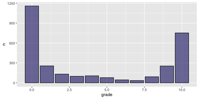
It would be reasonable to expect a gaussian-like distribution here, with a rounded peak somewhere between 3 and 7, tailing off on either side. Instead, we see nearly the opposite, with peaks at 0 and 10, and a shallow u-shaped distribution between. In the world of online reviews, especially for games, this sadly predictable behavior. Here some domain expertise is helpful…
Review Bombing
Despite ACNH’s metacritic score of 90% (making it one of the highest rated games of 2020 in the eyes of professional critics), its user reviews average just 55%. Players critical of the limits placed on all but the first player to start the game have resorted to review bombing:
“an Internet phenomenon in which large groups of people leave negative user reviews online for a published work, most commonly a video game or a theatrical film, in an attempt to harm the sales or popularity of a product, particularly to draw attention to an issue with the product or its vendor,” - Wikipedia.
The graph above clearly depicts this adolescent behavior, where the “haters” and “fanboys” have squared off to show their ire and support, respectively. This is something to keep in mind throughout the project.
Cleaning and Feature Engineering
For the purposes of this project it is also important to have a good
sense of what is found in the review text field. Samples of review text
were pulled for both positive (grade > 8) and negative (grade < 3)
observations and inspected. In doing so I noticed that longer entries
tended to include repeated text and end with the word “Expand.” These
problems were likely introduced during the scraping process. I also
noticed that some entries are not in English.
After some light initial cleanup of the text field, a new rating
column was added to label each review based on the grade. In order to
use binary classification methods, rating was set to “good” for values
greater than 5.0 and “bad” otherwise. This cutoff point was chosen based
on the average user review of 5.5, but it also seems natural. The
remaining cleanup of text data is done as part of the
Tokenization process, described below.
Final Exploration
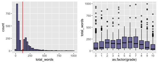
Two final plots were created to complete my exploration. First, the number of words per review was visualized using a histogram. The discontinuity in the resulting graph gives further evidence of problems with the scraped data. Otherwise, this result is as expected, with most reviews being relatively short (less than 75 words), but some users have submitted nearly 1,000 words! The red vertical line shows the average of 120.95 words per review.
Next, I looked for obvious relationships between grade and review
length using a box and whiskers plot. The number of outliers increases
with more extreme reviews, which seems to follow my intuition that
reviewers scoring the game very high or very low are more prone to
support their scores with extended rants / raves.
Train-Test Split
Lastly, the data was split into training and testing sets using the
customary 75/25 split. Training data will be used to fit the model and
tune the hyperparameters. Test data is reserved for final evaluation of
the best model to estimate its performance on new, unseen data. The
split was stratified by rating to ensure that the training and test
sets were balanced on the response variable. The splits are summarized
below.
##   rating count percent source
## 1    bad  1369   60.84  train
## 2   good   881   39.16  train
## 3    bad   456   60.88   test
## 4   good   293   39.12   test
Experiments
Null, Naive Bayes, Support Vector Machine, and Logistic (Lasso) Regression models are built and evaluated on both training and test data. The Null model is used to establish baseline performance metrics. The others were chosen for their performance on sparse data, a key characteristic of natural language problems that results from tokenization of the input data.
Tokenization
Tokenization is the process of converting the input text data into a format suitable for training ML algorithms. While many approaches are used, the method I used covers the essential steps. It begins with splitting the raw strings into tokens based on a combination of whitespace, punctuation, and other factors. I will use word tokens, as is the most common practice, but tokens can be characters, groups of words (n-grams), etc.
The resulting token list is filtered down using a list of stop words to remove elements with little predictive value. The reduced list is then sorted by frequency and the top 500 tokens are converted to “term frequency-inverse document frequency”, or TFIDF format. According to the documentation, TFIDF is the product of term frequency, the number of times each token appears in each observation, and the inverse document frequency, a measure of how informative a word is based on its rarity). Together these assess the overall value of each token. Finally, the TFIDF values are normalized.
These steps are implemented in the tidymodels::recipe defined below:
review_rec <- recipe(rating ~ text, data = review_train) %>%
  step_tokenize(text) %>%
  step_stopwords(text) %>%
  step_tokenfilter(text, max_tokens = 500) %>%
  step_tfidf(text) %>%
  step_normalize(all_predictors())
This recipe of preprocessing steps will be shared by all model worflows.
When applied to the training data, the result is a table with 2,250 rows
(one per observation), and 501 columns (one per token, plus the response
rating). An extract is shown below for the tokens “access”, “account”,
and “accounts”.
##   rating tfidf_text_access tfidf_text_account tfidf_text_accounts
## 1    bad        -0.1447401         -0.2129978          -0.1330606
Method 0 - Null Model Baseline
To establish a performance baseline, a Null Model was first constructed.
This trivial case predicts the majority class for all observations.
Based on the prior stratification statistics, we should expect 60.8%
accuracy classifying as bad.
The tidymodels framework was used to define a model specification and
workflow (including the Tokenization recipe described
above), fit the training data and generate predictions using 10-fold
cross-validation, collect the results, and generate the following
confusion matrix.
##           Truth
## Prediction bad good
##       bad  137   89
##       good   0    0
As expected, all predictions use the majority class, bad, and the
resulting accuracy is 60.8%. Note that only a single fold’s worth of
predictions are included in this result. Using the same model to make
predictions for all test data results in the following confusion matrix.
##           Truth
## Prediction bad good
##       bad  456  293
##       good   0    0
Here again the accuracy is 60.9%. The train and test accuracy match in this case because the split was stratified on the response. The Null Model is more accurate than the proverbial coin flip (50%), providing a useful point of comparison for the other models.
Method 1 - Naive Bayes
The first non-trivial model is a Naive Bayes classifier, which uses conditional probabilities to make predictions based on per-class statistics. This method is commonly used for text classification because it is fast, simple, and well-suited to sparse, high-dimensional data. I expect it to perform better than the baseline, but not as well as more sophisticated models to follow.
The same method was used to train the model, generate predictions, and collect metrics. Here we generate a Receiver Operator Characteristics (ROC) curve based on the results of each cross-validation fold.
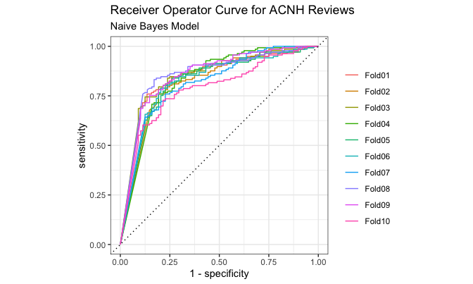
This shows the true positive rate (aka recall, aka sensitivity) on the
vertical axis vs. the false positive rate (aka
(1-\text{specificity})). While the end points are pinned at [0, 0]
and [1, 1], ideal curves are close to the top left, where true
positives are common and false positives are rare. The area under the
ROC curve, or ROC-AUC value, is a useful summary statistic. Values of
ROC-AUC less than 0.5 perform worse than a random guess, and the max
value is 1.0.
The corresponding confusion matrix for a representative cv fold is given below. The average cross-validation accuracy is 74.0%.
##           Truth
## Prediction bad good
##       bad  124   48
##       good  13   41
This is an improvement over the Null Model, but it is clearly better at
predicting bad reviews than good ones. When used to generate
predictions for all test data, the confusion matrix looks similar.
##           Truth
## Prediction bad good
##       bad  418  156
##       good  38  137
As expected, the Naive Bayes model performs better than the baseline but there is still room for improvement. The test set accuracy of 74.1% suggests that we are not overfitting this model.
Method 2 - Support Vector Machine
The Support Vector Machine model is a significantly more sophisticated method. As discussed in class this semester, SVMs work by finding hyperplanes that optimize class boundaries. A radial basis function (RBF) kernel is used to allow for nonlinearity, where the hyperparameter (\sigma) controls model complexity.
The processed used in this case is the same as above, with one notable
addition. A range of values for rbf_sigma are tested using
grid_regular() to find the optimal model. This results in 22,500
predictions: 10 cross-validation folds x 10 levels for sigma x 2,250
training observations. Unfortunately, the SVM solver does not return
prediction probabilities that are required to build a ROC curve. The
plot below shows accuracy, sensitivity, and specificity as a function of
(\sigma).
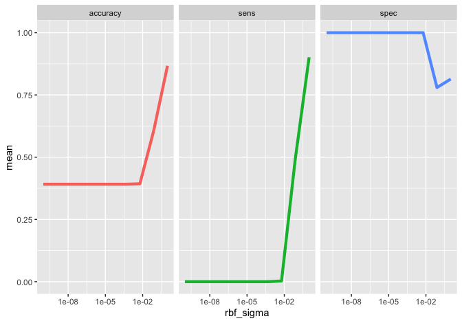
These curves can be used to select the best value of rbf_sigma for our
purposes. The top three models, based on training accuracy, are given
below.
# best accuracy for the training data
show_best(svm_grid, "accuracy")[1:3, ]
## # A tibble: 3 x 7
##   rbf_sigma .metric  .estimator  mean     n  std_err .config
##       <dbl> <chr>    <chr>      <dbl> <int>    <dbl> <chr>
## 1   1       accuracy binary     0.867    10 0.00650  Preprocessor1_Model10
## 2   0.0774  accuracy binary     0.606    10 0.0136   Preprocessor1_Model09
## 3   0.00599 accuracy binary     0.393    10 0.000786 Preprocessor1_Model08
From this we see that mean accuracy is maximized when (\sigma = 1.0). Honestly, this result seems fishy to me, but I was unable to find fault with the method. Using the optimal parameter value the model was fit using all training data and tthe following predictions were generated for the test set.
##           Truth
## Prediction bad good
##       bad  409   47
##       good  47  246
This looks quite good. Accuracy is 87.4% and the positive and negative predictive value is more balanced. It is easy to see why SVMs are a go-to tool for natural language processing.
Method 3 - Logistic Regression
The fourth and final method uses Logistic Regression with L1
regularization (i.e. lasso) to control model complexity. A range of
values are tested for the penalty parameter, adjusting the amount of
regularization applied. The resulting ROC curve is plotted below.
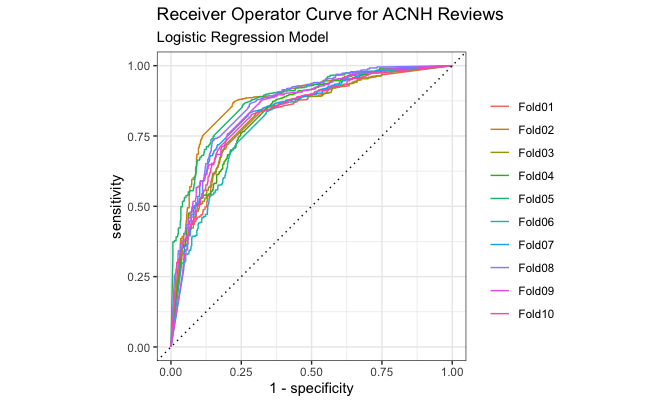
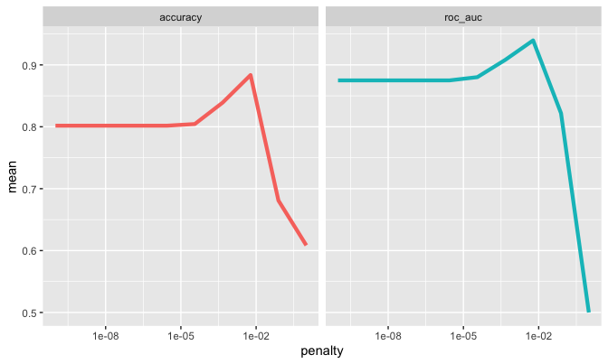
These curves bend closer to the top left corner than the Naive Bayes model, supporting our expectation that this is a better model. As with the SVM model, key metrics are plotted vs the hyperparameter of interest, and the top three models are listed by accuracy.
## # A tibble: 3 x 7
##     penalty .metric  .estimator  mean     n std_err .config
##       <dbl> <chr>    <chr>      <dbl> <int>   <dbl> <chr>
## 1 0.00599   accuracy binary     0.884    10 0.00534 Preprocessor1_Model08
## 2 0.000464  accuracy binary     0.839    10 0.00800 Preprocessor1_Model07
## 3 0.0000359 accuracy binary     0.804    10 0.00931 Preprocessor1_Model06
The top model listed, with accuracy 88.4, has a ROC AUC score of 0.94. Applying the optimal model to the test set yields the following confusion matrix.
##           Truth
## Prediction bad good
##       bad  417   52
##       good  39  241
The final accuracy here is 87.9%, slightly better than what was obtained with the SVM model.
Summarize Analysis
Beginning with the trivial Null Model, the increasing complexity of each subsequent method resulted in improved results. The accuracy on training and test data is summarized below for all models.
##   Model TrnAcc TstAcc
## 1  Null  60.80  60.90
## 2    NB  74.00  74.10
## 3   SVM  86.71  87.40
## 4    LR  88.36  87.90
With its marginally improved accuracy and reasonably balanced positive / negative predictive power the Logistic Regression model seems the best choice in this exercise. My concerns about the SVM’s grid search results give me even more confidence in this choice.
Further Exploration
As a final step I adopted the following code from Julia Silge’s ACNH
blog post. It uses the vip package to assess the relative importance
of predictor variables. This provides valuable insights into both how
the model works and the concepts that drive user sentiment about the
game.
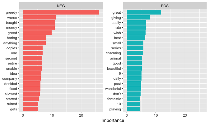
From this we can see that bad reviews are driven by the words “greedy,” “copies,” and “second,” all of which relate to the outrage over game limitations we discussed before. On the other hand, good reviews focus on the game being “great,” “beautiful,” and “charming,” among other similarly positive descriptors.
Conclusion
Text sentiment analysis is a valuable tool with many applications. This project gave me a first taste of the process, methods, and tools. It is a deep, fast moving topic that draws from diverse knowledge areas, making it a challenge to master despite the intuitive concepts.
Now that I have a broad understanding, future efforts to more deeply understand best practices for the front-end methods, including preprocessing, feature engineering, stop words, and tokenization, would likely yield the most dramatic improvements. Some specific improvements that I identified during this project include:
- Make it multi-class with 3-5 classifications, e.g. good / ok / bad
- Improve the quality of the data to minize / eliminate scraping errors
- Experiment with different stop word lists, which tend to be domain specific
- Experiment with the tokenizing approach, trying n-grams of various length
- Use clustering and/or association rules to identify groups of words that relate to user sentiment
- Expand the tuning grid parameters, including
max_tokensand other preprocessing variables - Try neural net and/or deep neural net models, which are very popular for NLP
In short, I’ve only scratched the surface of what is possible with this project. It has been a valuable effort and great capstone to the class.
References
- Mäntylä, Mika V., et al. “The Evolution of Sentiment Analysis—A Review of Research Topics, Venues, and Top Cited Papers.” Computer Science Review, vol. 27, Feb. 2018, pp. 16–32, doi:10.1016/j.cosrev.2017.10.002.
- Silge, Julia. Supervised Machine Learning Case Studies in R! · A Free Interactive Course. https://supervised-ml-course.netlify.app/. Accessed 21 Oct. 2020.
- —. Supervised Machine Learning for Text Analysis in R. https://smltar.com/. Accessed 21 Oct. 2020.
- —. Tidy Modeling with R. https://www.tmwr.org/. Accessed 21 Oct. 2020.
- Silge, Julia, and Emil Hvitfeldt. Predictive Modeling with Text Using Tidy Data Principles. https://emilhvitfeldt.github.io/useR2020-text-modeling-tutorial/. Accessed 2 Dec. 2020.